Probability distribution

Lore & Background

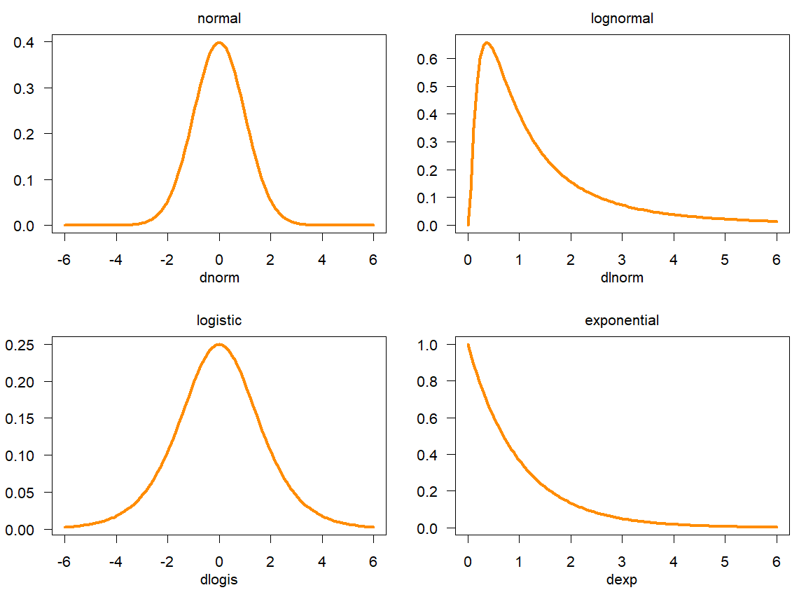
In probability theory and statistics, a probability distribution describes how probabilities are assigned to the possible results of a random phenomenon—more precisely, to events, which are sets of possible outcomes of a probabilistic experiment. Informally, a probability distribution tells us how likely different results are. Formally, it is a probability measure: a function that assigns probabilities to events in a way that satisfies the axioms of probability. Probability distributions are closely linked to random variables. A random variable is a function that assigns a value to each outcome of a probabilistic experiment; it induces a probability distribution on the set of values it can take. For example, the result of a coin toss can be represented by a random variable X that equals 1 for heads and 0 for tails. If the coin is fair, this distribution assigns probability 1/2 to X = 1 and probability 1/2 to X = 0. In practice, probability distributions are often described by functions such as cumulative distribution functions, probability mass functions, or probability density functions. Which description is used depends on the nature of the distribution: probability mass functions are used for discrete distributions, while probability density functions are used for many continuous distributions. Probability distributions that occur frequently or have special theoretical importance are often given specific names.

Reader's Guide

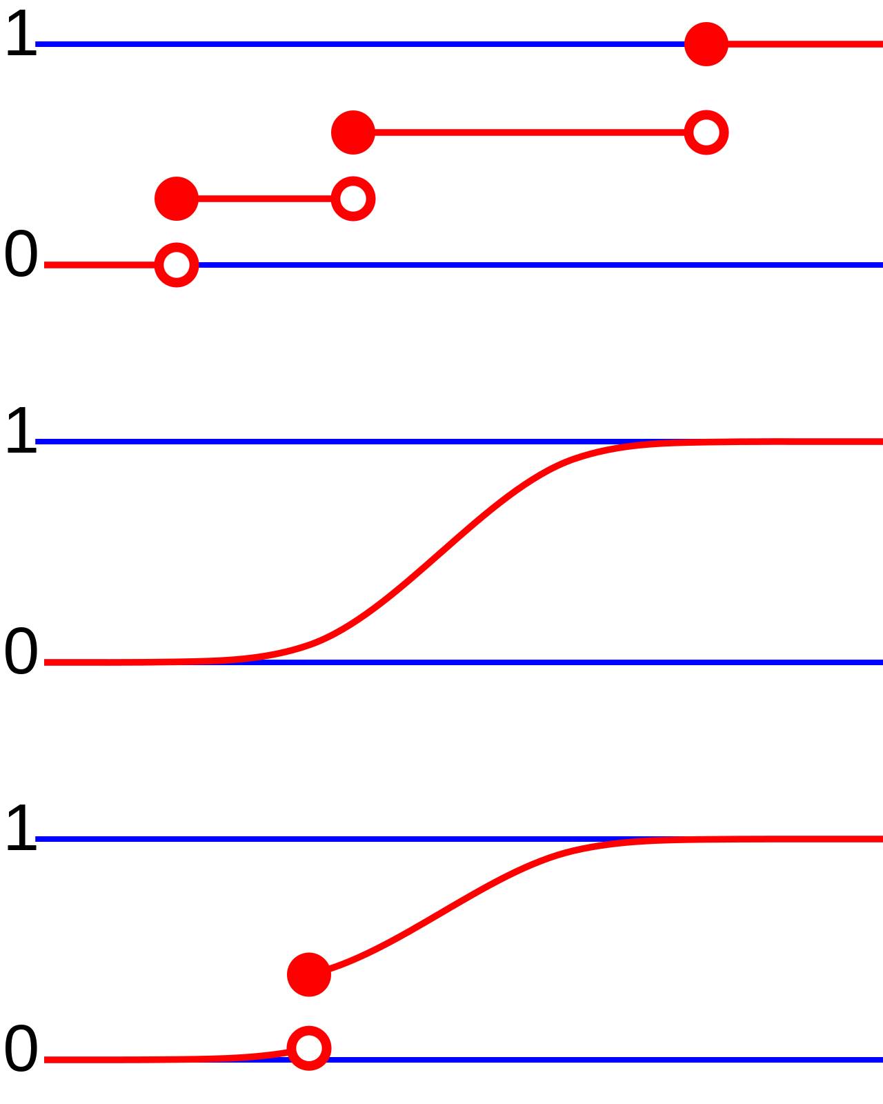
Probability distributions are fundamental to probability theory and statistics, providing the formal framework for quantifying uncertainty in random phenomena. They allow the assignment of probabilities to events—subsets of the sample space—and are essential for modeling everything from coin flips to continuous measurements like weight. The distinction between discrete and continuous distributions is key: discrete distributions use probability mass functions to assign probabilities to individual outcomes, while continuous distributions use probability density functions, where any single outcome has probability zero but intervals can have positive probability. The cumulative distribution function describes the probability that a random variable is no larger than a given value. By linking random variables to probability measures via pushforward measures, probability distributions enable rigorous statistical inference and are the basis for many named distributions used across science and engineering.

Did You Know?

• A probability distribution is formally a probability measure that satisfies the axioms of probability.
• For a fair coin, the probability distribution assigns probability 1/2 to heads and 1/2 to tails.
• Probability mass functions are used for discrete distributions, while probability density functions are used for many continuous distributions.
• The cumulative distribution function describes the probability that a random variable is no larger than a given value.

The Mathematical Core

The Poisson distribution is a discrete probability model that quantifies how likely it is to observe exactly k occurrences within a fixed interval, given that events arrive at a known, constant average rate and each event is independent of when the previous one happened. Its probability mass function takes the elegant form of λ to the power k, multiplied by e to the negative λ, all divided by k factorial, where k ranges over zero, one, two, and so on. The single parameter λ, which must be a positive real number, simultaneously determines both the mean and the variance of the distribution—a notable property that simplifies modeling considerably. When a problem provides an average event rate r rather than a total expected count, the formula adapts naturally by substituting λ with the product of r and the interval length t. This flexibility makes the distribution a workhorse for any scenario involving a large pool of potential events, each individually rare, where one wishes to count how many actually materialize during a specified window.

A Contested Legacy of Naming

The distribution bears the name of French mathematician Siméon Denis Poisson, who lived from 1781 to 1840. He introduced it in his 1837 treatise on the probability of judgments in criminal and civil matters, where he theorized about the number of wrongful convictions in a given country by examining random variables that count events over a fixed time interval. Yet the story does not end there. As early as 1711, Abraham de Moivre had derived similar results in his work on the measurement of chance in games of fortune. This makes the Poisson distribution a textbook case of Stigler's law, which observes that scientific discoveries are rarely named after their original discoverers. Some authors have argued on this basis that the distribution ought to carry de Moivre's name instead. The model's early practical uptake came in 1860, when Simon Newcomb applied it to count the number of stars found within a unit of space, and again in 1898, when Ladislaus Bortkiewicz demonstrated that the frequency of Prussian soldiers accidentally killed by horse kicks conformed remarkably well to the Poisson pattern.

From Call Centers to Cosmic Impacts

The distribution finds natural expression in a strikingly wide range of counting problems. A call center that receives an average of three calls per minute, with independent arrivals across disjoint intervals, will see between one and four calls in any given minute roughly seventy-seven percent of the time, while zero or five-or-more calls account for the remaining twenty-three percent. Radioactive decay events observed over a fixed period serve as a classic motivating example. On a grander scale, the number of meteorites exceeding one meter in diameter that strike Earth within a year can be modeled this way, as can the count of laser photons registering on a detector during a particular interval. In everyday contexts, the distribution captures how many students in a cohort achieve either very low or very high exam marks. In materials science, it describes the locations of defects and dislocations within a solid. What unites these examples is the underlying structure: a vast number of possible individual events, each with a small probability of occurring, whose aggregate count over a defined window follows the Poisson law.

Beyond the Time Axis: Spatial and Dimensional Reach

Although the Poisson distribution is most commonly introduced in the context of events accumulating over a time interval, its reach extends well beyond one dimension. The same mathematical framework applies when counting occurrences within a specified area or volume, effectively generalizing the concept of a fixed interval into higher-dimensional space. Two-dimensional spatial examples include the scatter of asteroid impact sites across Earth's surface and the distribution of tree locations within a forest. Three-dimensional examples encompass the placement of imperfections inside a bulk material. In each case, the independence assumption and the constant mean rate translate directly into the spatial domain. The distribution also occupies a distinguished position in the broader theory of discrete-stable distributions, underscoring its foundational role in probability. The requirement that events in disjoint sub-intervals remain independent is a key structural condition; when this holds, as in the call-center scenario where two non-overlapping minutes do not influence each other, the Poisson model provides an exact description rather than merely an approximation.

Gallery