Principal component analysis

Lore & Background

It was later independently developed and named by Harold Hotelling in the 1930s. Depending on the field, it is also called the discrete Karhunen–Loève transform in signal processing, the Hotelling transform in multivariate quality control, proper orthogonal decomposition in mechanical engineering, empirical orthogonal functions in meteorological science, and other names across disciplines.

Reader's Guide

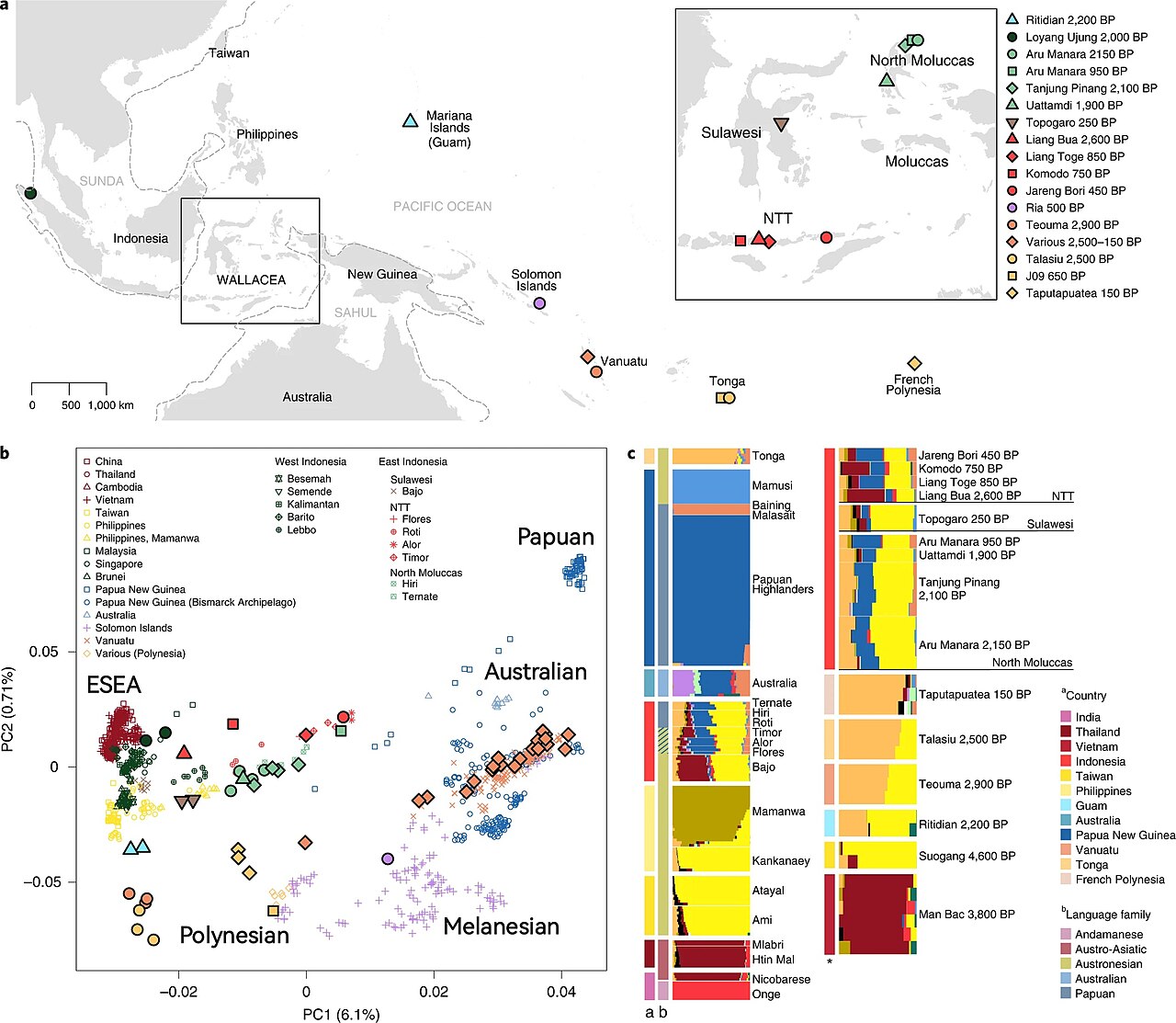
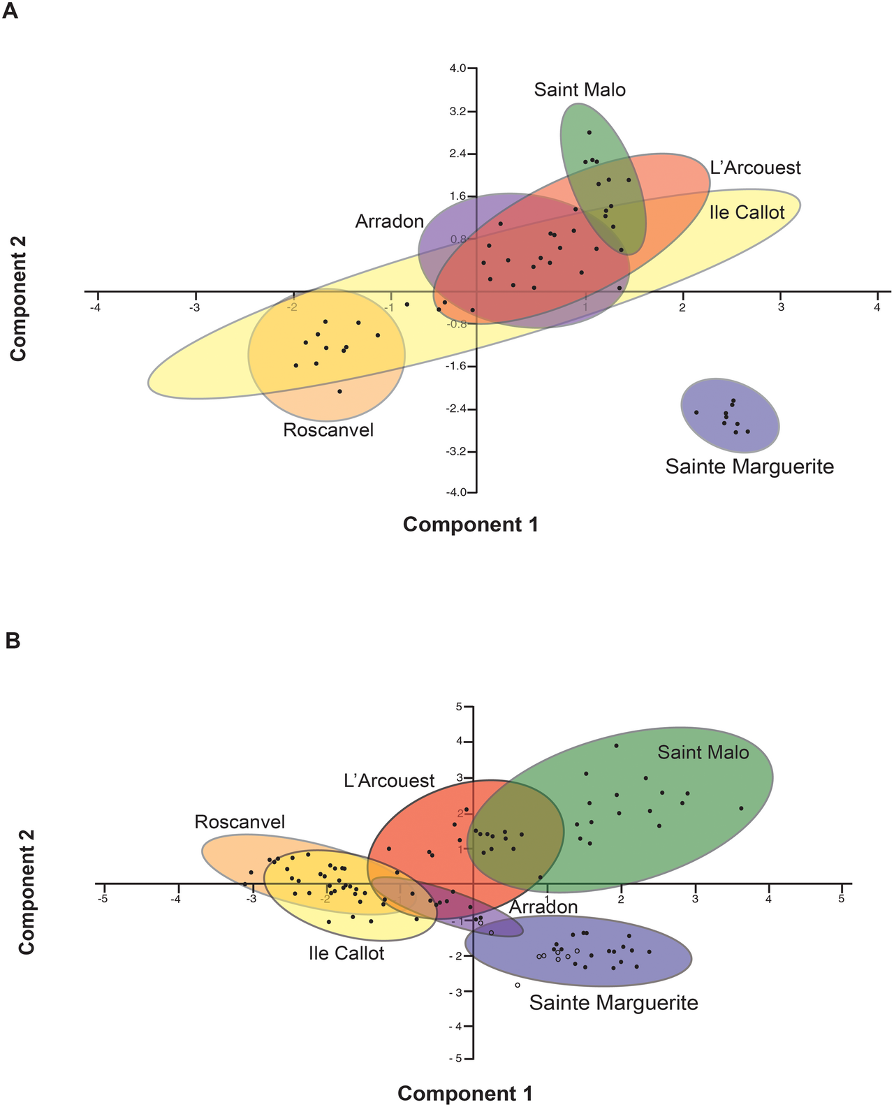
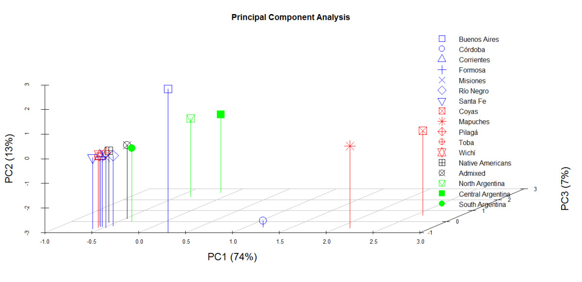
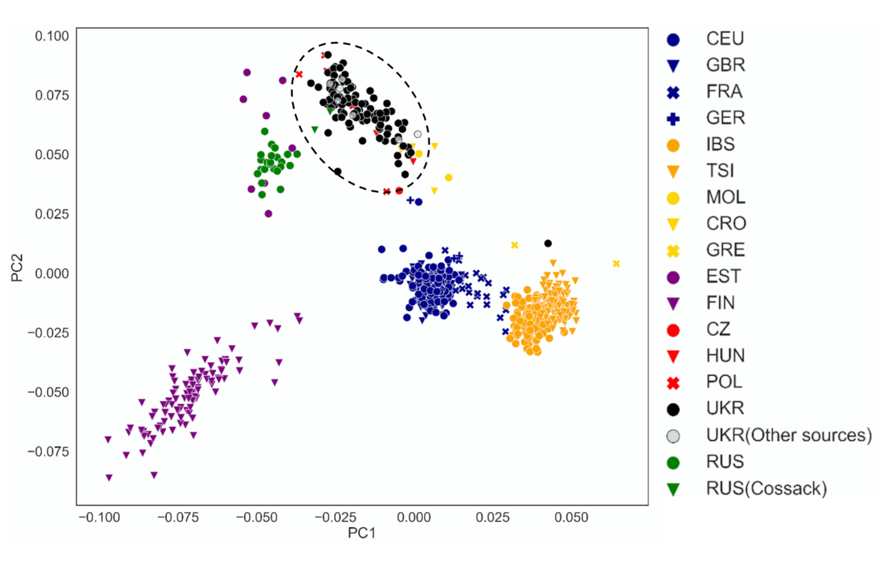
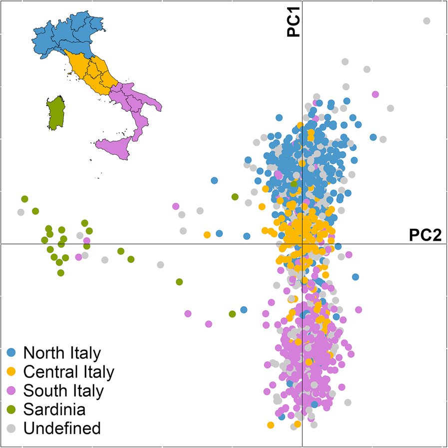
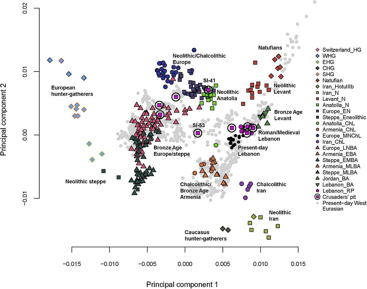
Principal component analysis is a foundational technique for reducing the dimensionality of datasets while preserving as much variance as possible. It works by finding a sequence of orthogonal unit vectors—the principal components—that best fit the data by minimizing the average squared perpendicular distance from points to each line. The first principal component explains the most variance, and each subsequent component explains the most variance orthogonal to the previous ones. Computationally, principal components are eigenvectors of the data's covariance matrix, often obtained via eigendecomposition or singular value decomposition. PCA is widely used in fields such as population genetics, microbiome studies, and atmospheric science. It is the simplest eigenvector-based multivariate analysis and is closely related to factor analysis and canonical correlation analysis. Many studies use the first two principal components to plot data in two dimensions and visually identify clusters. Biplots and scree plots are used to interpret PCA findings.

Did You Know?

• The first principal component maximizes the variance of the projected data.
• Principal components are eigenvectors of the data's covariance matrix.
• PCA is also known as the discrete Karhunen–Loève transform in signal processing.

The Variance-Chasing Engine

Principal component analysis operates as a linear dimensionality reduction technique that reorients an entire dataset onto a fresh coordinate system. At its heart, the method constructs a sequence of unit vectors, each one representing the direction of a line that best fits the data while remaining strictly orthogonal to every vector that came before it. Best fit here carries a precise meaning: the chosen direction minimizes the average squared perpendicular distance from all data points to that line. The first component captures the greatest possible variance among all linear combinations of the original variables, and each subsequent component extracts the most remaining variance after the preceding components have been accounted for. Mathematically, these directions turn out to be the eigenvectors of the data's covariance matrix, which means practitioners typically compute them through eigendecomposition of that covariance matrix or, equivalently, singular value decomposition of the raw data matrix. The resulting set of mutually orthogonal vectors forms an orthonormal basis in which the individual dimensions of the data become linearly uncorrelated, and PCA stands as the simplest member of the eigenvector-based multivariate analysis family.

One Method, a Dozen Names

Few statistical tools have accumulated as many aliases as principal component analysis. Karl Pearson first introduced the technique in 1901, framing it as a statistical analogue of the principal axis theorem from mechanics. Decades later, Harold Hotelling independently developed and gave the method its now-familiar name in the 1930s. Yet across the scientific landscape, the same mathematical operation wears a different hat in nearly every discipline. Signal-processing engineers call it the discrete Karhunen–Loève transform, while quality-control specialists refer to it as the Hotelling transform. Mechanical engineers know it as proper orthogonal decomposition, and meteorologists working with atmospheric data invoke empirical orthogonal functions, a term popularized by Lorenz in 1956. In linear algebra it surfaces as the singular value decomposition of a data matrix, a technique itself dating to the last quarter of the nineteenth century, or as the eigenvalue decomposition of the matrix X transpose times X. Researchers in noise and vibration call it spectral decomposition, structural-dynamics specialists use empirical modal analysis, and others have labeled it quasiharmonic modes or empirical eigenfunction decomposition. Even the Eckart–Young theorem points back to the same underlying eigenvector machinery.

The Ellipsoid Intuition

Rather than viewing PCA as an abstract algebraic procedure, one can picture it as fitting a p-dimensional ellipsoid around a cloud of data points. Each axis of that ellipsoid corresponds to one principal component, and the length of an axis directly reflects how much variance the data exhibit along that direction; a short axis signals little spread, a long one signals a great deal. To locate those axes in practice, the analyst first centers every variable by subtracting its observed mean from each value, so that all columns of the data matrix carry a zero empirical mean. The next step is to compute the covariance matrix of these centered values and then extract its eigenvalues and eigenvectors. After normalizing each orthogonal eigenvector into a unit vector, the collection of mutually perpendicular unit vectors defines the ellipsoid's axes. In this new basis the covariance matrix becomes diagonal, with the diagonal entries giving the variance along each axis. The fraction of total variance captured by any one component is simply its eigenvalue divided by the sum of all eigenvalues. Biplots and scree plots then provide visual summaries that help researchers interpret which components matter most.

From Genetics to the Atmosphere

Although PCA was born as a general-purpose linear algebra tool, its reach extends far beyond pure mathematics. In population genetics, microbiome research, and atmospheric science, analysts routinely apply the method to distill complex, high-dimensional measurements into a handful of interpretable axes. The technique is especially valuable when many of the original variables are highly correlated with one another, because PCA condenses them into an independent set that preserves the dominant patterns of variation. A common practical use is to take just the first two principal components and project the data onto a two-dimensional plane, making it possible to visually spot clusters of closely related observations. PCA also sits in a family of related multivariate methods: factor analysis, which layers additional domain-specific assumptions about underlying structure and solves eigenvectors of a slightly different matrix; canonical correlation analysis, which optimally describes cross-covariance between two separate datasets rather than variance within a single one; and robust or L1-norm-based variants that have been proposed to handle atypical observations more gracefully. In every case, the shared thread is the extraction of eigenvectors from a covariance-like structure.

Gallery